Researcher degrees of freedom in phonetic research
Timo B. Roettger
Department of Linguistics, Northwestern University, Evanston, United States
timo.roettger@northwestern.edu
Abstract
Every data analysis is characterized by a multitude of decisions, so-called “researcher degrees
of freedom” (Simmons, Nelson, & Simonsohn, 2011), that can affect its outcome and the conclusions
we draw from it. Intentional or unintentional exploitation of researcher degrees of
freedom can have dramatic consequences for our results and interpretations, increasing the
likelihood of obtaining false positives. It is argued that quantitative phonetics faces a large
number of researcher degrees of freedom due to its scientific object, speech, being inherently
multidimensional and exhibiting complex interactions between multiple co-varying layers. A
Type-I error simulation is presented that demonstrates the severe false error inflation when exploring
researcher degrees of freedom. It is argued that, combined with common cognitive fallacies,
unintentional exploitation of researcher degrees of freedom introduces strong bias and
poses a serious challenge to quantitative phonetics as an empirical science. This paper discusses
potential remedies for this problem including adjusting the threshold for significance, drawing
a clear line between confirmatory and exploratory analyses via preregistered reports, open,
honest and transparent practices in communicating data analytical decisions, and direct replications.
Keywords
false positive, methodology, preregistration, replication, reproducibility speech production, statistical
analysis
Acknowledgment
I would like to thank Aviad Albert, Eleanor Chodroff, Emily Cibelli, Jennifer Cole, Tommy
Denby, Matt Goldrick, James Kirby, Nicole Mirea, Limor Raviv, Shayne Sloggett, Lukas Soenning,
Mathias Stoeber, Bodo Winter, and two anonymous reviewers for valuable feedback on
earlier drafts of this paper. All remaining errors are my own.
1. Introduction
In our endeavor to understand human language, phoneticians and phonologists explore speech
behavior, generate hypotheses about aspects of the speech transmission process, and collect
and analyze suitable data in order to eventually put these hypotheses to the test. We proceed to
the best of our knowledge and capacities, striving to make this process as accurate as possible,
but, as in any other scientific discipline, this process can lead to unintentional misinterpretations
of our data. Within a scientific community, we need to have an open discourse about such
misinterpretations, raise awareness of their consequences, and find possible solutions to them.
In the most widespread framework of statistical inference, null hypothesis significance testing,
one common misinterpretation of data is a false positive, i.e. erroneously rejecting a null
hypothesis (Type I error)1. When undetected, false positives can have far reaching consequences,
potentially leading to bold theoretical claims which may misguide future research.
These types of misinterpretations can be persistent through time because our publication apparatus
does neither incentivize publishing null results nor direct replication attempts, biasing the
scientific record towards novel positive findings. As a result, there may be a large number of
null results in the “file drawer” that will never see the light of day (e.g. Sterling, 1959).
False positives can have many causes. One factor that has received little attention is the
so called “garden of forking paths” (Gelman & Loken, 2014) or what Simmons, Nelson, and Simonsohn (2011) call “researcher degrees of freedom”. Data analysis - that is, the path we chose
from the raw data to the results section of a paper - is a complex process. We can look at data
from different angles and each way to look at them may lead to different methodological and
analytical choices. The potential choices in the process of data analysis are collectively referred
to as researcher degrees of freedom. Said choices, however, are usually not specified in advance
but are commonly made in an ad hoc fashion, after having explored several aspects of the
data and analytical choices. In other words, they are data-contingent rather than motivated on
independent, subject-matter grounds. This is often not an intentional process but a result of
cognitive biases. Intentional or not, exploiting researcher degrees of freedom can increase false
positives rates. This problem is shared by all quantitative scientific fields (Gelman & Loken, the specific characteristics of phonetic analyses.
1 There are other errors that can happen and that are important to discuss. Most closely related to the
present discussion are Type II (Thomas et al., 1985), Type M, and Type S errors (Gelman & Carlin,
2014). Within quantitative linguistics, there are several recent discussions of these errors, see Kirby &
Sonderegger (2018), Nicenboim et al. (2018), Nicenboim & Vasishth (2016), Vasishth & Nicenboim
(2016). 2014; Simmons et al., 2011; Wichert et al., 2016), but has not been extensively discussed for
In this paper it will be argued that analyses in quantitative phonetics face a high number
of researcher degrees of freedom due to the inherent multidimensionality of speech behavior,
which is the outcome of a complex interaction between different meaning-signaling layers.
This article will discuss relevant researcher degrees of freedom in quantitative phonetic research,
reasons as to why exploiting researcher degrees of freedom is potentially harmful for
phonetics as a cumulative empirical endeavor, and possible remedies to these issues.
The remainder of this paper is organized as follows: In §2, I will review the concept of
researcher degrees of freedom and how they can lead to misinterpretations in combination with
certain cognitive biases. In §3, I will argue that researcher degrees of freedom are particularly
prevalent in quantitative phonetics, focusing on the analysis of speech production data. In §4, I
will present a simple Type-I error rate simulation, demonstrating that mere chance leads to a
large inflation of false-positives when we exploit common researcher degrees of freedom. In §5,
I will discuss possible ways to contain the probability of false positives due to researcher degrees
of freedom, discussing adjustments of the alpha level (§5.1), stressing the importance of a
more rigorous distinction between confirmatory and exploratory analyses (§5.2), preregistrations
and registered reports (§5.3), transparent reporting (§5.4), and direct replications (§5.5).
2. Researcher degrees of freedom
Every data analysis is characterized by a multitude of decision that can affect its outcome and,
in turn, the conclusions we draw from it (Gelman & Loken, 2014; Simmons et al., 2011;
Wichert et al., 2016). Among the decisions that need to be made during the process of learning
from data are the following: What do we measure? What predictors and what mediators do we
include? What type of statistical models do we use?
There are many choices to make and most of them can have an influence on the result that
we obtain. Researchers usually do not make all of these decisions prior to data collection: Rather
they usually explore the data and possible analytical choices to eventually settle on one
‘reasonable’ analysis plan which, ideally, yields a statistically convincing result. Depending on
the statistical framework we are operating in, our statistical results are affected by the number
of hidden analyses performed.
In most scientific papers, statistical inference is drawn by means of null hypothesis-significance-
testing (NHST, Gigerenzer et al., 2004; Lindquist, 1940). Because NHST is by a large margin the most common inferential framework used in quantitative phonetics, the present discussion
is conceived with NHST in mind. However, most of the arguments are relevant for
other statistical frameworks, too. Traditional NHST performs inference by assuming that the
null hypothesis is true in the population of interest. For concreteness, assume we are conducting
research on an isolated undocumented language and investigate the phonetic instantiation
of phonological contrasts. We suspect, the language has word stress, i.e. one syllable is phonologically
‘stronger’ than other syllables. We are interested in how word stress is phonetically
manifested and pose the following hypothesis:
(1) There is a phonetic difference between stressed and unstressed syllables.
NHST allows to compute the probability of observing a result at least as extreme as a test
statistic (e.g. t-value), assuming that the null hypothesis is true (the p-value). In our concrete
example, the p-value tells us the probability of observing our data or more extreme data, if
there really was no difference between stressed and unstressed syllables (null hypothesis). Receiving
a p-value below a certain threshold (commonly 0.05) is then interpreted as evidence to
claim that the probability of the data, if the null hypothesis was in fact true (no difference between
stressed and unstressed syllables), is sufficiently low.
Within this framework, any difference between conditions that yields a p-value below 0.05
is practically considered sufficient to reject the null hypothesis and claim that there is a difference.
However, these tests have a natural false positive rate, i.e. given a p-value of 0.05, there
is a 5% probability that our data accidentally suggests that the null can be refuted. When we
accept the arbitrary threshold of 0.05 to distinguish ‘significant’ from ‘non-significant’ findings
(which is under heated dispute at the moment, see Benjamin et al., 2018, see also §5.1), we
have to acknowledge this level of uncertainty surrounding our results which comes with a certain
base rate of false positives.
If, for example, we decide to measure only a single phonetic parameter (e.g. vowel duration)
to test the hypothesis in (1), 5% would be the base rate of false positives, given a p-value
of 0.05. However, this situation changes if we measure more than one parameter. For example,
we could test, say, vowel duration, average intensity, and average f0 (all common phonetic correlates
of word stress, e.g. Gordon & Roettger, 2017), amounting to three null hypothesis significance
tests. One of these analyses may turn out to be significant, yielding a p-value of 0.05 or
lower. We could go ahead and write our paper, claiming that stressed and unstressed syllables
are phonetically different in the language under investigation.
But this procedure increases the chances of finding a false positive. If n independent comparisons
are performed, the false positive rate would be 1− (1 −0.05)n instead of 0.05; three tests, for example, will produce a false positive rate of approximately 14% (i.e. 1 − 0.95 * 0.95
* 0.95 = 1 − 0.857 = 0.143). Why is that? Assuming that we could get a significant result
with a p-value of 0.05 by chance in 5% of cases, the more often we look at random samples,
the more often we will accidentally find a significant result (e.g. Tukey, 1953).
Generally, this reasoning can be applied to all researcher degrees of freedom. With
every analytical decision, with every forking path in the analytical labyrinth, with every researcher
degree of freedom, we increase the likelihood of finding significant results due to
chance. In other words, the more we look, explore, and dredge the data, the greater the likelihood
of finding a significant result. Exploiting researcher degrees of freedom until significance
is reached has been called out as harmful practices for scientific progress (John, Loewenstein, &
Prelec, 2012). Two often discussed instanced of such harmful practices is HARKing (Hypothesizing
After Results are Known, e.g. Kerr, 1998) and p-hacking (e.g. Simmons et al., 2011).
HARKing refers to the practice of presenting relationships that have been obtained after data
collection as if they were hypothesized in advance. P-hacking refers to the practice of hunting
for significant results in order to ultimately report these results as if confirming the planned
analysis. While such exploitations of researcher degrees of freedom are certainly harmful to the
scientific record, there are good reasons to believe that they are, more often than not, unintentional.
People are prone to cognitive biases. Our cognitive system craves for coherency, seeing patterns
in randomness (apophenia, Brugger, 2001); we weigh evidence in favor of our preconceptions
more strongly than evidence that challenges our established views (confirmation bias,
Nickerson, 1998); we perceive events as being plausible and predictable after they have occurred
(hindsight bias, Fischhoff, 1975).2 Scientists are no exception. For example, Bakker and
Wicherts (2011) analyzed statistical errors in over 250 psychology papers. They found that
more than 90% of the mistakes were in favor of the researchers’ expectations, making a nonsignificant finding significant. Fugelsang et al. (2004) investigated how scientists evaluate data
that are either consistent or inconsistent with prior expectations. They showed that when researchers
are faced with results that disconfirm their expectations, they are likely to blame the
methodology employed while results that confirmed their expectations were rarely critically
evaluated.
We work in a system that rewards and incentivizes positive results more than negative results
(John et al., 2012), so we have the natural desire to find a positive result in order to publish our findings. A large body of research suggests that when we are faced with multiple decisions,
we may end up convincing ourselves that the decision with the most rewarding outcome
is the most justified one (e.g. Dawson et al., 2002; Hastorf & Cantril, 1954). In light of the dynamic
interplay of cognitive biases and our current incentive structure in academia, having
many analytical choices may lead us to unintentionally exploit these choices during data analysis.
This can inflate the number of false positives.
2 See Greenland (2017) for a discussion of cognitive biases that are more specific to statistical analyses.
3. The garden of forking paths in quantitative phonetics
Quantitative phonetics is no exception to the discussed issues and may in fact be particularly at
risk because its very scientific object offers a considerable number of perspectives and decisions
along the data analysis path. The next section will discuss researcher degrees of freedom in
phonetics, and will, for exposition purposes, focus on speech production research. It turns out
that the type of data that we are collecting, i.e. acoustic or articulatory data, opens up many
different forking paths (for a more discipline-neutral assessment of researcher degrees of freedom,
see Wichert et al., 2016). I discuss the following four sets of decisions (see Fig. 1 for an
overview): choosing phonetic parameters (§3.1), operationalizing chosen parameters (§3.2),
discarding data (§3.3), and choosing speech-related independent variables (§3.4). These distinctions
are made for convenience and I acknowledge that there are no clear boundaries between
these four sets. They highly overlap and inform each other to different degrees.
Figure 1: Schematic depiction of decision procedure during data analysis that can lead
to an increased false positive rate. Along the first analysis pipeline (blue), decisions are
made as to what phonetic parameters are measured (§3.1), how they are operationalized
(§3.2), what data is kept and what data is discarded (§3.3) and what additional independent
variables are measured (§3.4). The results are statistically analyzed (which
comes with its own set of researcher degrees of freedom, see Wichert et al., 2016) and
interpreted. If the results are as expected and/or desired, the study will be published. If
not, cognitive biases facilitate reassessments of earlier analytical choices (red arrow) (or
a reformulation of hypotheses, i.e. HARKing), increasing the false positive rate.
3.1 Choosing phonetic parameters
When conducting a study on speech production, the first important analytical decision to test a
hypothesis is the question of operationalization, i.e. how to measure the phenomenon of interest.
For example, how do we measure whether two sounds are phonetically identical, whether
one syllable in the word is more prominent than others, or whether two discourse functions are
produced with different prosodic patterns? In other words, how to we quantitatively capture
relevant features of speech?
Speech categories are inherently multidimensional and vary through time. The acoustic
parameters for one category are usually asynchronous, i.e. appear at different points of time in
the unfolding signal and overlap with parameters for other categories (e.g. Jongman et al.,
2000; Lisker, 1986; Summerfield, 1984; Winter, 2014). If we zoom in and look at a well-researched
speech phenomenon such as the voicing distinction between stops in English, it turns
out that the distinction between voiced and voiceless stops can be manifested by many different
acoustic parameters such as voice onset time (e.g. Lisker & Abramson, 1963), formant transitions
(e.g. Benkí, 2001), pitch in the following vowel (e.g. Haggard et al., 1970), the duration
of the preceding vowel (e.g. Raphael, 1972), the duration of the closure (e.g. Lisker, 1957), as
well as spectral differences within the stop release (e.g. Repp, 1979). Even temporally dislocated
acoustic parameters correlate with voicing, for example, in the words led versus let, voicing
correlates can be found in the acoustic manifestation of the initial /l/ of the word (Hawkins
& Nguyen, 2004). These acoustic aspects correlate with their own set of articulatory configurations,
determined by a complex interplay of different supralaryngeal and laryngeal gestures, coordinated
with each other in intricate ways.
This multiplicity of phonetic cues exponentially grows if we look at larger temporal
windows as it is the case for suprasegmental aspects of speech. Studies investigating acoustic
correlates of word-level prominence, for example, have been using many different measurements
including temporal characteristics (duration of certain segments or subphonemic intervals),
spectral characteristics (intensity measures, formants, and spectral tilt), and measurements
related to fundamental frequency (f0) (Gordon & Roettger, 2017).
Looking at even larger domains, the prosodic expression of pragmatic functions can be
expressed by a variety of structurally different acoustic cues which can be distributed throughout
the whole utterance. Discourse functions are systematically expressed by multiple tonal
events differing in their position, shape, and alignment (e.g. Niebuhr et al., 2011). They can
also be expressed by global or local pitch scaling, as well as acoustic information within the
temporal or spectral domain (e.g. Cangemi, 2015; Ritter & Roettger, 2015; van Heuven & van
Zanten 2005).3 All of these dimensions are potential candidates for our operationalization and
therefore represent researcher degrees of freedom.
If we ask questions such as “is a stressed syllable phonetically different from an unstressed
syllable?”, out of all potential measures, any single measure has the potential to reject
the corresponding null hypothesis (there is no difference). But which measurement should we
pick? There are often many potential phonetic correlates for the relevant phonetic difference
under scrutiny. Looking at more than one measurement seems to be reasonable. However, looking
at many phonetic exponents to test a single global hypothesis increases the false error rate.
If we were to test 20 dimensions of the speech signal repeatedly, on average one of these tests
will, by mere chance, result in a spurious significant result (at a 0.05 alpha level). We obviously
have justified preconceptions about which phonetic dimensions may be good candidates
for certain functional categories, informed by a long list of references. However, while these
preconceptions can certainly help us make theoretically-informed decisions, they may also bear
the risk for ad hoc justifications of analytical choices that happen after having explored researcher
degrees of freedom.
One may further object that dimensions of speech are not independent of each other,
i.e. many phonetic dimensions co-vary systematically. Such covariation between multiple
acoustic dimensions can, for example, result from originating from the same underlying articulatory
configurations. For example, VOT and onset f0, the fundamental frequency at the onset
of the vowel following the stop, are systematically co-varying across languages, which has been
argued to be a biomechanical consequence of articulatory and/or aerodynamic configurations
(Hombert, Ohala, & Ewan, 1979). Löfqvist et al. (1989) showed that when producing voiceless
consonants, speakers exhibit higher levels of activity in the cricothyroid muscle and in turn
greater vocal fold tension. Greater vocal fold tension is associated with higher rates of vocal
fold vibration leading to increased f0. Since VOT and onset f0 are presumably originating from
the same articulatory configuration, one could argue that we do not have to correct for multiple
testing when measuring these two acoustic dimensions. However, as will be shown in §4,
correlated measures lead to false positive inflation rates that are nearly as high as in independent
multiple tests (see also von der Malsburg & Angele, 2017).
3 Speech is not an isolated channel of communication, it co-occurs in rich interactional contexts. Beyond acoustic and articulatory dimensions, spoken communication is accompanied by non-verbal modalities such as body posture, eye gaze direction, head movement and facial expressions, all of which have been shown to contribute to comprehension and may thus be considered relevant parameters to measure (Cummins, 2012; Latif et al., 2014; Prieto et al., 2015; Rochet-Capellan et al., 2008; Yehia et al., 1998).
3.2 Operationalizing chosen parameters
The garden of forking paths does not stop here. There are many different ways to operationalize
the dimensions of speech that we have chosen. For example, when we want to extract specific
acoustic parameters of a particular interval of the speech signal, we need to operationalize
how to decide on a given interval. We usually have objective annotation procedures and clear
guidelines that we agree on prior to the annotation process, but these decisions have to be considered
researcher degrees of freedom and can potentially be revised after having seen the results
of the statistical analysis.
Irrespective of the actual annotation, we can look at different acoustic domains. For example,
a particular acoustic dimension such as duration or pitch can be operationalized differently
with respect to its domain and the way it is assessed: In their survey of over a hundred
acoustic studies on word stress correlates, Gordon and Roettger (2017) encountered dozens of
different approaches how to quantitatively operationalize f0, intensity, and spectral tilt as correlates
of word stress. Some studies took the whole syllable as a domain, others targeted the
mora, the rhyme, the coda or individual segments. Specific measurements for f0 and intensity
included the mean, the minimum, the maximum, or even the standard deviation over a certain
domain. Alternative measures included the value at the midpoint of the domain, at the onset
and offset of the domain, or the slope between onset and offset. The measurement of spectral
tilt was also variegated. Some studies measured relative intensity of different frequency bands,
where the choice of frequency bands varied considerably across studies. Yet other studies measured
relative intensity of the first two harmonics.
Similarly, time-series data such as pitch curves, formant trajectories or articulatory
movements have been analyzed as sequences of static landmarks (“magic moments”, Vatikiotis-
Bateson, Barbosa & Best, 2014), with large differences across studies regarding the identity and
the operationalization of these landmarks. For example, articulatory studies looking at intragestural
coordination commonly measure gestural onsets, displacement metrics, peak velocity,
the onset and offset of gestural plateaus, or stiffness (i.e. relating peak velocity to displacement).
Alternatively, time-series data can be analyzed holistically as continuous trajectories,
differing with regard to the degrees of smoothing applied (e.g. Wieling, 2018).
In multidimensional datasets such as acoustic or articulatory data, there may be thousands
of sensible analysis pathways. Beyond that, there are many different ways to process
these raw measurements with regard to relevant time windows and spectral regions of interest;
there are many possibilities of transforming or normalizing the raw data or smoothing and interpolating trajectories.
3.3 Discarding data
Setting aside the multidimensional nature of speech and assuming that we actually have a priori
decided on what phonetic parameters to measure (see 3.1) and how to measure and process
them (see 3.2), we are now faced with additional choices. We let two annotators segment the
speech stream and annotate the signal according to clearly specified segmentation criteria. During
this process, the annotators notice noteworthy patterns that either make the preset operationalization
of the acoustic criteria ambiguous or introduce possible confounds.
The segmentation process may be difficult due to undesired speaker behavior, e.g. hesitations,
disfluencies, or mispronunciations. There may be issues related to the quality of the recording
such as background noise, signal interference, technical malfunctions or interruptive
external events (something that happens quite frequently during field work).
Another aspect of the data that may strike us as problematic when we extract phonetic
information are other linguistic factors that could interfere with our research question. Speech
consists of multiple information channels including acoustic parameters that distinguish words
from each other and acoustic parameters that structure prosodic constituents into rhythmic
units, structure utterances into meaningful units, signal discourse relations or deliver indexical
information about the social context. Dependent on what we are interested in, the variable use
of these information channels may interfere with our research question. For example, a speaker
may produce utterances that differ in their phrase-level prosodic make-up. In controlled production
studies, speakers often have to produce a very restricted set of sentences. Speakers may
for whatever reason (boredom, fatigue, etc.) insert prosodic boundaries or alter the information
structure of an utterance, which, in turn, may drastically affect the phonetic form of other parts
of the signal. For example, segments of accented words have been shown to be phonetically enhanced,
making them longer, louder, and more clearly articulated (e.g. Cho & Keating, 2009;
Harrington et al., 2000). Related to this point, speakers may use different voice qualities, some
of which will make the acoustic extraction of certain parameters difficult. For example, if we
were interested in extracting f0, parts of the signal that are produced with a creaky voice may
not be suitable; or if we were interested in spectral properties of the segments, parts of the signal
produced in falsetto may not be suitable.
It is reasonable to ‘clean’ the data and remove data points that we consider as not desirable,
i.e. productions that diverge from the majority of productions (e.g. unexpected phrasing,
hesitations, laughter, etc.). These undesired productions may interfere with our research hypothesis
and may mask the signal, i.e. make it less likely to find systematic patterns. We can exclude these data points in a list-wise fashion, i.e. subjects who exhibit a certain amount of
undesired behavior (set by a certain threshold) may be entirely excluded. Alternatively, we can
exclude trials on a pair-wise level across levels of a predictor. We can also simply exclude problematic tokens on a trial-by-trial basis. All of these choices change our final data set and, thus,
may affect the overall result of our analysis.
To exemplify the point, let us assume recorded utterances exhibit prosodic variation:
Sometimes the target word carries a pitch accent and sometimes it is deaccented. It is easily
justifiable to only look at the accented tokens, as the segmental cues are likely to be enhanced
in these contexts. It is equally justifiable to do the opposite, only looking at deaccented variants
as this should make a genuine lexical contrast more difficult to obtain and, in turn, makes the
refutation of the null hypothesis (i.e. there is no difference) more difficult.
3.4 Choosing independent variables
Often, subsetting the data or exclusion of whole clusters of data can have impactful consequences,
as we would discard a large amount of our collected data. Instead of discarding data
due to unexpected covariates, we can add these covariates as independent variables to our
model. In our example, we could include the factor of accentuation as an interaction term into
our analysis to see whether the investigated effect may interact with accentuation. If we either
find a main effect of syllable position on our measurements or an interaction of with accentuation,
we would probably proceed and refute the null hypothesis (there is no difference between
stressed and unstressed syllables). This rational can be applied to external covariates, too. For
example, in prosodic research, researchers commonly add the sex of their speakers to their
models, either as a main effect or an interaction term, so as to control for the large sex-specific
f0 variability. Even though this reasoning is justified by independent factors, it represents a set
of researcher degrees of freedom.
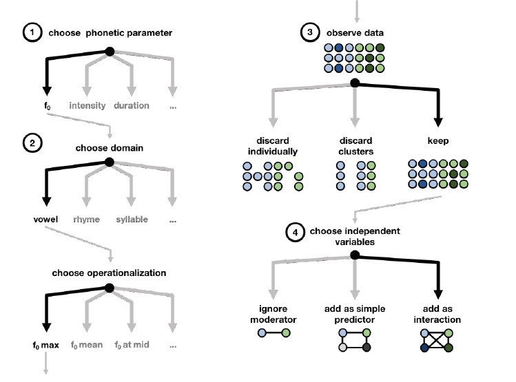
Figure 2: Schematic example of forking analytical paths as described in §3. First, the
researchers choose from a number of possible phonetic parameters (1), then they choose
in what temporal domain they measure this parameter and how they operationalize it
(2). After extracting the data, the researchers must decide how to deal with dimension
of speech that are orthogonal to what they are primarily interested in (say the difference
between stressed and unstressed syllables: blue vs. green dots, 3). For example, speakers
might produce words either with or without a pitch accent (light vs. dark dots). They
can discard undesired observations (e.g. discard all deaccented target words), discard
clusters (e.g. discard all contrasting pairs that contain at least one deaccented target
word), or keep the entire data set. If they decide to keep them, the question arises as
whether to include these moderators or not and if so whether to include them as a simple
predictor of add them to an interaction term (4). Note that these analytical decisions
are just a subset of all possible researcher degrees of freedom at each stage.
To summarize, the multidimensional nature of speech offers a myriad of different ways
to look at our data. It allows us to choose dependent variables from a large pool of candidates;
it allows us to measure the same dependent variable in alternative ways; and it allows us to
preprocess our data in different ways by for example normalization or smoothing algorithms.
Moreover, the complex interplay of different levels of speech phenomena introduced the possibility
to correct or discard data during data annotation in a non-blinded fashion; it allows us to
measure other variables that can be used as covariates, mediators or moderators. These variables
could also enable further exclusion of participants (see Figure 2 for a schematic example).
While there are often good reasons to go down one forking path rather than another,
the sheer amount of possible ways to analyze speech comes with the danger of exploring many
of these paths and picking those that yield a statistically significant result. Such practices, exactly
because they are often unintentional, are problematic because they drastically increase
the rate of false positives.
It is important to note that these researcher degrees of freedom are not restricted to speech
production studies. Within more psycholinguistically oriented studies in our field, we can for
example examine online speech perception by monitoring eye movements (e.g. Tanenhaus et
al., 1995) or hand movements (Spivey et al., 2005). There are many different informative relationships between these measured motoric patterns and aspects of the speech signal. For example,
in eye tracking studies, we can investigate different aspects of the visual field (foveal, parafoveal,
peripheral), we can look at the number and time course of different fixations of a region
(e.g. first, second, third), the duration of a fixation or the sum of fixations before exiting / entering
a particular region (see von der Malsburg & Angele, 2017, for a discussion).
More generally, the issue of researcher degrees of freedom is relevant for all quantitative
scientific disciplines (see Wichert et al., 2016). As of yet, we have not discussed much of the
analytical flexibility that is specific to statistical modeling: There are choices regarding the
model type, model architecture, and the model criticism procedure, all of which come with
their own set of researcher degrees of freedom. Note that having these choices is not problematic
per se, but unintentionally exploring these choices before a final analytical commitment has
been made may inflate false positive rates. Depending on the outcome and our preconception
of what we expect to find, confirmation and hindsight bias may lead us to believe that there
are justified ways to look at the data in one particular way, until we reach a satisfying (significant)
result. Again, this is a general issue in scientific practices and applies to other disciplines,
too. However, given the multidimensionality of speech as well as the intricate interaction of
different level of speech behavior, the possible unintentional exploitation of researcher degrees
of freedom is particularly ubiquitous in our field. To demonstrate the possible severity of the issue, the following section presents a simulation that simulates false positive rates based on
analytical decisions that speech production studies face commonly.
4. Simulating researcher degrees of freedom exploitation
In this section, a simulation is presented which shows that exploiting researcher degrees of
freedom increases the probability of false positives, i.e. erroneously rejecting the null hypothesis.
The simulation was conducted with R (R Core Team, 2016)4 in order to demonstrate the effect
of two different sets of researcher degrees of freedom: Testing multiple dependent variables
and adding a binomial covariate to the model (for similar simulations, see e.g. Barr et al.,
2013; Winter, 2011, 2015). Additionally, the correlation between dependent variables is varied
with one set of simulations assuming three entirely independent measurements (r =0), and one
set of simulations assuming measurements that are highly correlated with each other (r =0.5).
The script to reproduce these simulations is publicly available here (osf.io/6nsfk)5.
The simulation is based on the following dummy experiment: A group of researchers analyzes
a speech production data set to test the hypothesis that stressed and unstressed syllables
are phonetically different from each other. They collect data from 64 speakers producing words
with either stress category. Speakers vary regarding the intonational form of their utterances
with approximately half of the speakers producing a pitch accent on the target word and the
other half deaccenting the target word.
As opposed to a real-world scenario, we know the true underlying effect, since we draw
values from a normal distribution around a mean value that we specify. In the present simulation,
there is no difference between stressed and unstressed syllables in the “population”, i.e.
values for stressed and unstressed syllables are drawn from the same underlying distribution.
However, due to chance sampling, there are always going to be small differences between
stressed and unstressed syllables in any given sample. Whether the word carried an accent or
not is also randomly assigned to data points. In other words, there is no true effect of stress,
neither is there an effect of accent on the observed productions.
4 The script utilizes the MASS package (Venables & Ripley, 2002) and the tidyverse package
(Wickham, 2017).
5 The simulation was inspired by Simmons et al.’s (2011) simulation which is publicly available
here: https://osf.io/a67ft/.
We simulated 10,000 datasets and tested for the effect of stress on dependent variables
under different scenarios. In our dummy scenarios, researchers explored following researcher
degrees of freedom:
(i) Instead of measuring a single dependent variable to refute the null hypothesis, the
dummy researchers measured three dependent variables (say, intensity, f0 and duration). Measuring
multiple aspects of the signal is common practice within the phonetic literature across
phenomena. In fact, measuring only three dependent variables is probably on the lower end of
what researchers commonly do. However, phonetic aspects are often correlated, some of them
potentially being generated by the same biomechanical mechanisms. To account for this aspect
of speech, these variables were generated as either being entirely uncorrelated or being highly
correlated with each other (r =0.5).
(ii) The dummy researchers explored the effect of the accent covariate and tested
whether inclusion of this variable as a main effect or as an interacting term with stress yields a
significant effect (or interaction effect). Accent (0,1) was randomly assigned to data rows with
a probability of 0.5, that is there is no inherent relationship with the measured parameters.
These two scenarios correspond to researcher degrees of freedom 1 and 4 in Fig. 1 and
2. Based on these scenarios, the dummy researchers ran simple linear models on respective dependent
variables with stress as a predictor (and accent as well as their interaction in scenario
ii). The simulation counts the number of times, the researchers would obtain at least one significant
result (p-value <0.05) exploring the garden of forking paths described above.
This simulation (as well as the scenario it is based on) is admittedly a simplification of
real-world scenarios and might therefore not be representative. As discussed above, the number
of researcher degrees of freedom are manifold in phonetic investigations, therefore any simulation
has to be a simplification of the real state of affairs. For example, the simulation is based
on a regression model for a between-subject design, therefore not taking within-subject variation
into account. It is thus important to note that the ‘true’ false positive rates in any given experimental
scenario are not expected to be precisely as reported, or that the relative effects of
the various researcher degrees of freedom are similar to those found in the simulation. The true
false positive rates may differ from those reported here. Despite these necessary simplifications,
the generated numbers can be considered very informative and are intended to illustrate the
underlying principles of how exploiting researcher degrees of freedom can impact the false positive
rate.
We should expect about 5% significant results for an alpha level of 0.05 (the commonly
accepted threshold in NHST). Knowing that there is no stress contrast in our simulated population,
any significant result is by definition a false positive. Given the proposed alpha level, we
thus expect that on average 1 out of 20 studies will show a false positive. Fig. 3 illustrates the
results based on 10,000 simulations.
Figure 3: The x axis depicts the proportion of studies for which at least one attempted
analysis was significant at a 0.05 level. Light grey bars indicate the results for uncorrelated
measures, dark grey bars indicate results for highly correlated measures (r = 0.5).
Results were obtained for running three separate linear models for each dependent variable
(row 1-3); for running one linear model with the main effect only, one model
allowing for covariance with an accent main effect, and one model with an analysis of
covariance with an accent interaction (row 4, a significant effect is reported if the effect
of the condition or its interaction with accent was significant in any of these analyses).
Row 5-6 combine multiple dependent variables with adding a covariate. The dashed
line indicates the expected false positive base rate of 5%.
The baseline scenario (only one measurement, no covariate added) provides the expected base
rate of false positives (5%, see row 1 in Fig. 3). Departing from this baseline, the false positive
rate increases substantially (row 2-6). Looking at the results for the uncorrelated measurements
first (light grey bars), results of the simulation indicate that as the researchers measure three dependent variables (rows 2-3), e.g. three possible acoustic exponents, they obtain a significant
effect in 14.6% of all cases. In other words, by testing three different measurements, the falseerror
rate increases by a factor of almost 3. When researchers explore the possibility of the effect
under scrutiny co-varying with a random binomial co-variate, they obtain a significant effect
in 11.9% of cases, increasing the false-error rate by a factor of 2.3. These numbers may
strike one as rather low but they are based on only a small number of researcher degrees of
freedom. In real-world scenarios, some of these choices are entirely random but potentially informed
by the researcher’s preconceptions and expectations, potentially clouded by cognitive
biases.
Moreover, we usually walk through the garden of forking paths and unintentionally exploit
multiple different researcher degrees of freedom at the same time. If the dummy researchers
combine measure three different acoustic exponents and run additional analyses for the
added covariate the false error rate increases to 31.5%, and increases by a factor of over 6, i.e.
the false-error rate is more than six times larger than our agreed rate of 5%.
One might argue that the acoustic measurements that we take are highly correlated, making
the choice between them not as impactful since they measure the same thing. To anticipate
this remark, the same simulations were run with highly correlated measurements (r =0.5, see
dark grey bars in Fig. 3). Although the false-positive rate is slightly lower than for the uncorrelated
measures, we still obtain large number of false positives. If the dummy researchers measure
three different acoustic exponents and run additional analyses for the added covariate, the
false error rate is 28%. Thus, despite the measurements being highly correlated, the false error
rate is still very high (see also Malsburg & Angele 2017 for a discussion of eye-tracking data).
In order to put these numbers into context, imagine a journal that publishes 10 papers per issue
and each paper reports only one result. Given the described scenario above, 3-4 papers of this
issue would report a false positive.
Keep in mind that the presented simulation is necessarily a simplification of real-world
data sets. The true false positive rates might differ from those presented here. However, even
within a simplified scenario, the present simulation serves as a proof of concept that exploiting
researcher degrees of freedom can impact the false positive rate quite substantially.
Another limitation of the present simulation (and of most simulations of this nature) is
that it is blind to the direction of the effect. Here, we counted every p-value below our set alpha
level as a false positive. In real-world scenarios, however, one could argue that we often
have directional hypotheses. For example, we expect unstressed syllables to exhibit ‘significantly’ shorter durations/lower intensity/lower f0, etc. It could be argued that finding a significant
effect going into the ‘wrong’ direction is potentially less likely to be considered trustworthy
evidence (i.e. unstressed syllables being longer). However, due to cognitive biases such as
hindsight bias (Fischhoff, 1975) and overconfident beliefs in the replicability of significant results
(Vasishth, Mertzen, & Jäger, 2018) the subjective expectedness of effect directionality
might be misleading.
The discussed issues are general issues of data analysis operating in a particular inferential
framework and they are not specific to phonetic sciences. However, we need to be aware of
these issues and we need to have an open discourse about them. It turns out that one of the aspects
that makes our scientific object so interesting, the complexity of speech, can pose a methodological
burden. But there are ways to substantially decrease the risk of producing false positives.
5. Possible remedies
The demonstrated false-positive rates are not an inevitable fate. In the following, I will discuss
possible strategies to elude the threat posed by researcher degrees of freedom, focusing on five
different topics: I discuss the possibility of adjusting the alpha level as a way to reduce false
positives (§5.1). Alternatively, I propose that drawing a clear line between exploratory and confirmatory
analyses (§5.2) and committing to researcher degrees of freedom prior to data collection
with preregistered protocols (§5.3) can limit the number of false positives. Additionally, a
valuable complementary practice may lie in open, honest and transparent reporting on how
and what was done during the data analysis procedure (§5.4). While transparency cannot per
se limit the exploitation of researcher degrees of freedom, it can facilitate their detection. Finally,
it is argued that direct replications are our strongest strategy against false positives and
researcher degrees of freedom (§5.5).
5.1 Adjusting the significance threshold
The increased false positive rates as discussed in this paper are closely linked to null hypothesis
significance testing which, in its contemporary form, constitutes a dichotomous statistical decision
procedure based on a preset threshold (the alpha level). At first glance, an obvious solution
to reduce the likelihood of obtaining false positives is to adjust the alpha level, either by
correcting it for relevant researcher degrees of freedom or by lowering the decision threshold
for significance a priori.
First, one could correct the alpha level as a function of the number of exploited researcher
degrees of freedom. This solution has mainly been discussed in the context of multiple comparisons,
in which the researcher corrects the alpha level threshold according to the number of
tests performed (Benjamini & Hochberg, 1995; Tukey, 1954). If we were to measure three
acoustic parameters to test a global null hypothesis, which can be refuted by a single statistically
significant result, we would lower the alpha level to account for three tests. These corrections
can be done for example via the Bonferroni or the Šidák method.6
One may object that corrections for multiple testing are not reasonable in the case of
speech production on the grounds that acoustic measures are usually correlated. In this case,
correcting for multiple tests may be too conservative. However, as demonstrated in §4 and discussed
by von der Malsburg & Angele (2017), multiple testing of highly correlated measures
leads to false positive rates that are nearly as high as for independent multiple tests. Thus, a
multiple comparisons correction is necessary even with correlated measures in order to obtain
the conventional false positive rate of 5%.
For the concrete simulation presented in §4, we could conservatively correct for the number
of tests that we have performed, e.g. correcting for testing three dependent variables. While
such corrections capture the simulated false positive rate for multiple tests on uncorrelated
measures well, they are too conservative to capture the false positive rates for scenarios in
which measures are correlated to different degrees. Simply correcting for multiple tests would
be too conservative in these cases.
Given the large analytical decision space that we have discussed above, it remains unclear
as to how much to correct the alpha level for individual researcher degree of freedom. Moreover,
given that speech production experiments usually yield a limited amount of data, strong
alpha level corrections can drastically inflate false negatives (Type II errors, e.g. Thomas et al.,
1985), i.e. erroneously accepting the null hypothesis. Alpha level correction does also not help
us detect exploitation of researcher degrees of freedom. If our dummy researchers have measured
20 different variables, but only report 3 of them in the published manuscript, correcting
the alpha level for the reported three variables is too anti-conservative.
6 One approach is to use an additive (Bonferroni) inequality: For n tests, the alpha level for each test is given by the overall alpha level divided by n. A second approach is to use a multiplicative inequality (Šidák): For n tests, the alpha level for each test is calculated by taking 1 minus the nth root of the complement of the overall alpha level.
Alternatively, one could pose a more conservative alpha level that we agree on within the
quantitative sciences a priori. Benjamin et al. (2018) recently made such a proposal, recommending
to lower our commonly agreed alpha level from p ≤ 0.05 to p ≤ 0.005. All else being
equal, lowering the alpha level will reduce the absolute number of false positives (e.g. in the
simulation above, we would only obtain around 0.5% to 3% of false positives across scenarios).
However, it has been argued that lowering the commonly accepted threshold for significance
potentially increases the risk of scientific practices that could harm the scientific record even
further (Amrhein & Greenland, 2018; Amrhein, Korner-Nievergelt, & Roth, 2017; Greenland,
2017; Lakens et al., 2018): In order to demonstrate a ‘significant’ result, studies would need
substantially larger sample sizes7, increasing the rate of false negatives. Requiring larger sample
sizes also leads to an increase in time and effort associated with a study (while possible academic
rewards remain the same), potentially reducing the willingness of researchers to conduct
direct replication studies even further (see §5.5, Lakens et al., 2018). Lowering the bar as to
what counts as significant is also unlikely to tackle issues such as p-hacking, HARKing, or publication
bias. Instead it might lead to an amplification of cognitive biases that justify exploration
of alternative analytical pipelines (Amrhein & Greenland, 2018; Amrhein, Korner-Nievergelt, &
Roth, 2017). In sum, although the adjustment of alpha levels appears to limit false positives, it
is not always clear how to adjust it and it might introduce other dynamics that potentially
harm the scientific record.
5.2 Flagging analyses as exploratory vs. confirmatory
One important remedy to tackle the issue of researcher degrees of freedom is to draw a clear
line between exploratory and confirmatory analyses, two conceptually separate phases in scientific
discovery (Box, 1976; Tukey, 1980). In an exploratory analysis, we observe patterns and
relationships which lead to the generation of concrete hypotheses as to how these observations
can be explained. These hypotheses can then be challenged by collecting new data (e.g. in controlled
experiments). Putting our predictions under targeted scrutiny helps us revising our theories
based on confirmatory analyses. Our revised models can then be further informed by additional
exploration of the available data. This iterative process of alternating exploration and
confirmation advances our knowledge. This is hardly any news to the reader. However, quantitative
research in science in general as well as in our field in particular often blurs the line between
these two types of data analysis.
7 E.g. achieving 80% power with an alpha level of 0.005, compared with an alpha level of 0.05, requires 70% larger sample sizes for between-subjects designs with two-sided tests (see Lakens et al., 2018).
Exploratory and confirmatory analyses should be considered complementary to each
other. Unfortunately, when it comes to publishing our work, they are not weighted equally.
Confirmatory analyses have a superior status, determining the way we frame our papers and
the way funding agencies demand successful proposals to look like. This asymmetry can have
harmful consequences which I have discussed already: HARKing and p-hacking. It may also incentivize
researchers to sidestep clear-cut distinctions between exploratory and confirmatory
findings. The publication apparatus forces our thoughts into a confirmatory mindset, while we
often want to explore the data and generate hypotheses. For example, we want to explore what
the most important phonetic exponents of a particular functional contrast are. We may not necessarily
have a concrete prediction that we want to test at this stage, but we want to understand
patterns in speech with respect to their function. Exploratory analyses are necessary to
establish standards as to how aspects of speech relate to linguistic, cognitive, and social variables.
Once we have established such standards, we can agree to only look at relevant phonetic
dimensions, reducing the analytical flexibility with regard to what and how to measure (§3.1-
3.2).
Researcher degrees of freedom mainly affect the confirmatory part of scientific discovery,
they do not restrict our attempts to explore our data. But claims based on exploration
should be cautious. After having looked at 20 acoustic dimensions, any seemingly systematic
pattern may be spurious. Instead, this exploratory step should generate new hypotheses which
we then can confirm or disconfirm using a new dataset. In many experiments, prior to data collection,
it may be simply not clear how a functional contrast may manifest itself phonetically.
Presenting such exploratory analyses as confirmatory may hinder replicability and may give a
false feeling of certainty regarding the results (Vasishth et al., 2018). In a multivariate setting,
which is the standard setting for phonetic research, there are multiple dimensions to the data
that can inform our theories. Exploring these dimensions may often be more valuable than just
a single confirmatory test of a single hypothesis (Baayen et al., 2017). These cases make the
conceptual line between confirmatory and exploratory analyses so important. We should explore
our data. Yes. Yet we should not pretend that we are testing concrete hypotheses when
doing so.
Although our academic incentive system makes drawing this line difficult, journals start
to become aware of this issue and have started to create incentives to publish exploratory analyses
explicitly (for example Cortex, see McIntosh, 2017). One way of ensuring a clear separation
between exploratory and confirmatory analyses are preregistrations and registered reports
(Nosek et al., 2018; Nosek & Lakens, 2014).
5.3 Preregistrations and registered reports
A preregistration is a time-stamped document in which researchers specify exactly how they
plan to collect their data and how they plan to conduct their confirmatory analyses. Such reports
can differ with regard to the details provided, ranging from basic descriptions of the
study design to detailed procedural and statistical specifications up to the publication of scripts.
Preregistrations can be a powerful tool to reduce researcher degrees of freedom because
researchers are required to commit to certain decisions prior to observing the data. Additionally,
public preregistration can at least help to reduce issues related to publication bias, i.e. the
tendency to publish positive results more often than null results (Franco et al., 2014; Sterling,
1959), as the number of failed attempts to reject a hypothesis can be tracked transparently (if
the studies were conducted).
There are several websites that offer services and / or incentives to preregister studies
prior to data collection, such as AsPredicted (AsPredicted.org) and the Open Science Framework
(osf.io). These platforms allow us to time-log reports and either make them publicly available
or grant anonymous access only to a specific group of people (such as reviewers and editors
during the peer-review process).
A particular useful type of preregistration is a peer-reviewed registered report, which an
increasing number of scientific journals adopted already (Nosek et al., 2018; Nosek & Lakens,
2014, see cos.io/rr for a list of journals that have adopted this model).8 These protocols include
the theoretical rationale of the study and a detailed methodological description. In other words,
a registered report is a full-fledged manuscript minus the result and discussion section. These
reports are then critically assessed by peer reviewers, allowing the authors to refine their methodological
design. Upon acceptance, the publication of the study results is in-principle guaranteed,
no matter whether the results turn out to provide evidence for or against the researcher’s
predictions.
For experimental phonetics, a preregistration or registered report would ideally include
a detailed description of what is measured and how exactly it is measured/operationalized, as
well as a detailed catalogue of objective inclusion criteria (in addition to other key aspects of
the method including all relevant researcher degrees of freedom related to preprocessing, postprocessing,
statistical modelling, etc. see Wichert et al., 2016). Committing to these decisions
prior to data collection can reduce the danger of unintentionally exploiting researcher degrees
of freedom.
8 Note that journals that are specific to quantitative linguistics have not adopted these practices yet.
At first sight, there appear to be several challenges that come with preregistrations (see
Nosek et al., 2018, for an exhaustive discussion). For example, after starting to collect data, we
might realize that our preset exclusion criteria do not capture an important behavioral aspect
of our experiment (e.g., some speakers may produce undesired phrase-level prosodic patterns
which we did not anticipate). These patterns, however, interfere with our research question.
Deviations from our data collection and analysis plan are common. In this scenario, we could
change our preregistration and document these changes alongside our reasons as to why and
when (i.e. after how many observations) we have made these changes. This procedure still provides
substantially lower risk of cognitive biases impacting our conclusions compared to a situation
in which we did not preregister at all.
Researchers working with corpora may object that preregistrations cannot be applied
to their investigations because their primary data has already been collected. But preregistration
of analyses can still be performed. Although, ideally, we limit researcher degrees of freedom
prior to having seen the data, we can (and should) preregister analyses after having seen
pilot data, parts of the study, or even whole corpora. When researchers generate a hypothesis
that they want to confirm with a corpus dataset, they can preregister analytic plans and commit
to how evidence will be interpreted before analyzing the data.
Another important challenge when preregistering our studies is predicting appropriate
inferential models. Preregistering a data analysis necessitates knowledge about the nature of
the data. For example, we might preregister an analysis assuming that our measurements are
normally distributed. After collecting our data, we might realize that the data has heavy right
tales, calling for a log-transformation, thus, our preregistered analysis might not be appropriate.
One solution to this challenge is to define data analytical procedures in advance that allow
us to evaluate distributional aspects of the data and potential data transformations irrespective
of the research question. Alternatively, we could preregister a decision tree. This may actually
be tremendously useful for people using hierarchical linear models (often referred to linear
mixed effects models). When using appropriate random effect structures (see Barr et al., 2013;
Bates et al., 2015), these models are known to run into convergence issues (e.g. Kimball et al.,
in press). To remedy such convergence issues, a common strategy is to drop complex random
effect terms incrementally (Bates et al., 2015). Since we do not know whether a model will
converge or not in advance, a concrete plan of how we reduce model complexity can be preregistered
in advance (e.g. see the preregistration of Roettger & Franke 2017 as an example).
Preregistrations and registered reports help us draw a line between the hypotheses we
intend to test and data exploration. Any exploration of the data beyond the preregistered reports
have to be considered as hypotheses-generating only. If we are open and transparent about this distinction and ideally publicly indicate where we draw the line between the two,
we can limit false positives due to researcher degrees of freedom exploitation in our confirmatory
analyses and commit more honestly to subsequent exploratory analyses.
5.4 Transparency
The credibility of scientific findings is mainly rooted in the evidence supporting it. We assess
the validity of this evidence by constantly reviewing and revising our methodologies, and by
extending and replicating findings. This becomes difficult, if parts of the process are not transparent
or cannot be evaluated. For example, it is difficult to evaluate whether exploitation of
researcher degrees of freedom is an issue for any given study, if the authors are not transparent
about when they made which analytical decisions. We end up having to trust the authors. Trust
is good, control is better. We should be aware and open about researcher degrees of freedom
and communicate this aspect of our data analyses to our peers as honestly as we can. If we
have measured ten phonetic parameters, we should provide this information; if we have run
different analyses based on different exclusion criteria, we should say so and discuss the results
of these analyses. An open, honest and transparent research culture is desirable. As argued
above, public preregistration can facilitate transparency of what analytical decisions we make
and when we have made them. Being transparent does of course not prevent p-hacking, HARKing
or other exploitations of researcher degrees of freedom but it makes these harmful practices
detectable.
For our field, transparency with regard to our analysis has many advantages (e.g.
Nicenboim et al., 2018).9 As analysis is subjective in the sense that it incorporates the researcher’s
beliefs and assumptions about a study system (McElreath, 2016) the only way to
make analyses objectively assessable is to be transparent about this aspect of empirical work.
Transparency then allows other researchers to draw their own conclusions as to which researcher
degrees of freedom were present and how they may have affected the original conclusion.
9 Beyond sharing data tables and analysis scripts, it would be desirable to share raw acoustic or articulatory files. However, making these types of data available relies on getting permission from participantsin advance (as acoustic data is inherently identifiable). If we collect their participants’ consents, making raw speech production data available to the community would greatly benefit evidence accumulation in our field. We can share these data on online repositories such as OSCAAR (the Online Speech/Corpora Archive and Analysis Resource: https://oscaar.ci.northwestern.edu/).
In order to facilitate such transparency, we need to agree on how to report aspects of
our analyses. While preregistrations and registered reports lead to better discoverability of researcher
degrees of freedom, they do not necessarily allow us to systematically evaluate them.
We need institutionalized standards, as many other disciplines have already developed. There
are many reporting guidelines that offer standards for reporting methodological choices (see
the Equator Network for an aggregation of these guidelines: http://www.equator-network.
org/). Systematic reviews and meta analyses such as Gordon and Roettger (2017) and
Roettger & Gordon (2017) can be helpful departure points to create an overview of possible analytical decisions and their associated degrees of freedom (e.g. what is measured; how it is
measured, operationalized, processed, and extracted; what data are excluded; when and how
are they excluded, etc.). Such guidelines, however, are only effective when a community agrees
on their value and applies them including journals, editors, reviewers, and authors.
5.5 Direct replications
The above discussed remedies help us to both limit the exploitation of researcher degrees of
freedom and make them more detectable, but none of these strategies is a bullet-proof protection
against false positives. To ultimately avoid the impact of false-positives on the scientific
record, we should increase our efforts to directly replicate previous research, defined here as
the repetition of the experimental methods that led to a reported finding.
The call for more replication is not original. Replication has always been considered a
tremendously important aspect of the scientific method (e.g. Campbell, 1969; Kuhn, 1962; Popper,
1934/1992; Rosenthal, 1991) and in recent coordinated efforts to replicate published results,
the social sciences uncovered unexpectedly low replicability rates, a state of affairs that
has been coined the ‘replication crisis’. For example, the Open Science Collaboration (2015)
tried to replicate 100 studies that were published in three high-ranking psychology journals.
They assessed whether the replications and the original experiments yielded the same result
and found that only about one third to one half of the original findings (depending on the definition
of replication) were also observed in the replication study. This lack of replicability is
not restricted to psychology. Concerns about the replicability of findings have been raised for
medical sciences (e.g. Ioannidis, 2005), neuroscience (Wager, Lindquist, Nichols, Kober, & van
Snellenberg, 2009), genetics (Hewitt, 2012), cancer research (Errington et al., 2014), and economics
(Camerer et al., 2016).
Most importantly, it is a very real problem for quantitative linguistics, too. For example,
Nieuwland et al. (2018) recently tried to replicate a seminal study by DeLong et al. (2005)
which is considered a landmark study for the predictive processing literature and which has been cited over 500 times. In their preregistered multi-site replication attempt (9 laboratories,
334 subjects), Nieuwland et al. were not able to replicate some of the key findings of the original
study.
Stack, James, & Watson (2018) recently failed to replicate a well-cited effect of rapid
syntactic adaptation by Fine, Jaeger, Farmer, and Qian (2013). After failing to find the original
effect in an extension, they went back and directly replicated the original study with appropriate
statistical power. They found no evidence for rapid syntactic adaptation.
Possible reasons for the above cited failures to replicate are manifold. As has been argued
here, exploitation of researcher degrees of freedom is one reasons why there is a large
number of false positives. Combined with other statistical issues such as low power (e.g. for recent
discussion see Kirby & Sonderegger, 2018; Nicenboim et al., 2018), violation of the independence
assumption (Nicenboim & Vasishth, 2016; Winter 2011, 2015), and the ‘significance’
filter (i.e. treating results publishable because p < 0.05 leads to overoptimistic expectations of
replicability, see Vasishth et al., 2018), it is to be expected that there are a large number of experimental
phonetic findings that may not stand the test of time.
The above replication failures sparked a tremendously productive discourse throughout
the quantitative sciences and led to quick methodological advancements and best practice recommendations.
For example, there are several coordinated efforts to directly replicate important
findings by multi-site projects such as the ManyBabies project (Frank et al., 2017) and
Registered Replication Reports (Simons, Holcombe, &, Spellman, 2014). These coordinated efforts
can help us put theoretical foundations on a firmer footing. However, the logistic and
monetary resources associated with such large-scale projects are not always pragmatically feasible
for everyone in the field.
Replication studies are not very popular because the necessary time and resource investment
are not appropriately rewarded in contemporary academic incentive systems (Koole &
Lakens, 2012; Makel, Plucker, & Hegarty, 2012; Nosek, Spies, & Motyl, 2012). Both successful
replications (Madden, Easley, & Dunn, 1995) and repeated failures to replicate (e.g., Doyen,
Klein, Pichon, & Cleeremans, 2012) are only rarely published, and if they are published they
are usually published in less prestigious outlets than the original findings. To overcome the
asymmetry between the cost of direct replication studies and the presently low academic payoff
for it, we as a research community must re-evaluate the value of direct replications. Funding
agencies, journals, editors, and reviewers should start valuing direct replication attempts, be it
successful replications or replication failures, as much as they value novel findings. For example,
we could either dedicate existing journal space for direct replications (e.g. as an article
type) or by creating new journals that are specifically dedicated to replication studies.
As soon as we make publishing replications easier, more researchers will be compelled
to replicate both their own work and the work of others. Only by replicating empirical results
and evaluating the accumulated evidence can we substantiate previous findings and extend
their external validity (Ventry & Schiavetti, 1986).
6. Summary and concluding remarks
This article has discussed researcher degrees of freedom in the context of quantitative phonetics.
Researcher degrees of freedom concern all possible analytical choices that may influence
the outcome of our analysis. In a null-hypothesis-significance testing framework of inference,
intentional or unintentional exploitation of researcher degrees of freedom can have a dramatic
impact on our results and interpretations, increasing the likelihood of obtaining false positives.
Quantitative phonetics faces a large number of researcher degrees of freedom due to its scientific
object being inherently multidimensional and exhibiting complex interactions between
many co-varying layers of speech. A Type-I error simulation demonstrated substantial false error
rates when combining just two researcher degrees of freedom such as testing more than one
phonetic measurement, and including a speech-relevant co-variate in the analysis. It has been
argued that combined with common cognitive fallacies, unintentional exploitation of researcher
degrees of freedom introduces strong bias and poses a serious challenge to quantitative
phonetics as an empirical science.
Several potential remedies for this problem have been discussed. When operating in the
NHST statistical framework, we can reconsider our preset threshold for significance, a strategy
that has been argued to come with its own set of shortcomings. Several alternative solutions
have been proposed (see Fig. 4).
Figure 4: Schematic depiction of decision procedure during data analysis that limits
false positives: Prior to data collection, the researcher commits to an analysis pipeline
via preregistration/registered reports, leading to a clear separation of confirmatory
(blue) and exploratory analysis (light green). The analysis is executed accordingly and
the results are interpreted with regard to the confirmatory analysis. After the confirmatory
analysis, the researcher can revisit the decision procedure and explore the data
(green arrow). The interpretation of the confirmatory analysis and potentially insights
gained from the exploratory analysis are published alongside an open and transparent
track record of all analytical steps (preregistration, code and data for both confirmatory
and exploratory analysis). Finally, either prior to publication or afterwards, the study is
directly replicated (dark green arrow) by either the same research group or independent
researchers in order to substantiate the results.
We should draw an explicit line between confirmatory and exploratory analyses. One way to
enforce such a clear line are preregistrations or registered reports, records of the experimental
design and the analysis plan, committed to prior to data collection and analysis. While preregistration
offers better detectability of researcher degrees of freedom, standardized reporting
guidelines and transparent reporting might facilitate a more objective assessment of these researcher
degrees of freedom by other researchers. Yet all of these proposals come with their
own limitations and challenges. A complementary strategy to limit false positives lies in direct
replications, a form of research that is not well rewarded within the present academic system.
We as a community need to be openly discussing such issues and find practically feasible
solutions to them. Possible solutions must not only be feasible from a logistic perspective
but should also avoid punishing rigorous methodology within our academic incentive system.
Explicitly labeling our work as exploratory, being transparent about potential bias due to researcher
degrees of freedom, or direct replication attempts may make it more difficult to be rewarded
for our work (i.e. by being able to publish our studies in prestigious journals). Thus,
authors, reviewers, and editors alike need to be aware of these methodological challenges. The
present paper was conceived in the spirit of such an open discourse. Thus, the single most powerful
solution to methodological challenges as described in this paper, is engaging in a critical
and open discourse about our methods and analyses.
7. References